1.2 The economic way of thinking

e.g. 1: Striking while it's hot [versus] Biding your time

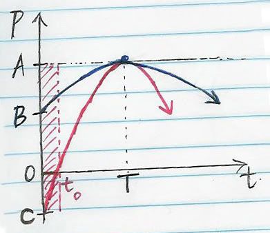
Take a look at this diagram.

- What the heck is that? (Also, it's a little crooked.)

Well, it is a [crookedly scanned] graph of opportunity versus time. But I used 'P' for prospect instead of 'O' for opportunity... 'cause, you know, 'O' looks like zero...

So I guess the model is something like P = R(t-T)² + A, where R ≺ 0, t ≥ 0,  and positive values of P are good and negative values of P are bad.

There are two curves: the blue one (1) and the red one (2) that depict possible scenarios when it comes to opportunities.

Firstly, when does t = 0? There are several possible explanations:

• When you first meet the person;
• When you begin the pursuit, not necessarily marked by any physical move;
• When you initiate something, ie. a physical move;
• When the other party initiates;
• Also, the sucky one, when the other party commits the second one and you are most likely unaware.
• - (Others I may have not thought of)

Alright, time to start analysing the graphs.

NB: Each individual target will have their own curve where R varies accordingly.

Curve 1: This curve is displaced to the right and starts off positive with an intercept at point B showing that from the very 'beginning', you're good to go. However, it is widely accepted that acting too fast is often seen as desperate/tacky and you are wiser to wait before proceeding. Hence, the curve rises to a universal point of maximum prospect*, P = A, at point (T, A), before logically falling again as it passes T units of time and eventually goes into the negative.

Curve 2: The difference here lies in the coefficient R, which determines the gradient of the slope, and hence the window of opportunity(W), and furthermore, the duration of the no-go zone (0 ≺ t ≺ to).
As shown in the graph, it is definitely a possibility that from the very start, P is a negative value (point C) and hence, any action is at your own expense. This lasts until t = t0, where P = 0 at the intercept, and then the window of opportunity (ie. for all values of t where P > 0) opens up, but for a shorter duration as the higher value of R has shrunk the window's range of values. 

So what is R? It can be referred to as the magnitude of risk.

     So as ↑R → ↓W

Finally, a common point to be drawn from these models is that as t → ∞, prospects will inevitably reach negative. ie. Do not wait too long.

BUT, *the quadratic model discussed is a very standard and very general take on the concept. For some people, there may not have been a window of opportunity at all for you, and the maximum prospect has already occured below the t axis. Furthermore, there very well may be individuals whose opportunity curve is a sin(t) or a loge(t), and perhaps even asymptotal components.

So, I will conclude this example with a special treat for Marco anybody that is interested.

[Nevermind, I couldn't be bothered parodying an extended response from my Methods 07 Checkpoints, took me long enough to write this up already. Maybe some other time.]

NEXT TIME: More stuff

EDIT: Wow. This is relevant, fascinating, and well its the Gradual Report, so it goes a little wrong in the middle somewhere. Also, it's about economics so time to slap it onto the end of the post as an edit. http://www.youtube.com/watch?v=4upRZ4TEdVM

Labels: puaeconomics, PUE8800